Ensemble Comparison
Preparation
First we import the necessary modules.
from pensa.comparison import *
from pensa.features import *
from pensa.statesinfo import *
import numpy as np
Then we load the structural features as described in the previous tutorial:
sim_a_rec = read_structure_features(
    "traj/condition-a_receptor.gro",
    "traj/condition-a_receptor.xtc"
)
sim_b_rec = read_structure_features(
    "traj/condition-b_receptor.gro",
    "traj/condition-b_receptor.xtc"
)
sim_a_rec_feat, sim_a_rec_data = sim_a_rec
sim_b_rec_feat, sim_b_rec_data = sim_b_rec
Relative Entropy
Here we compare the two ensembles using measures for the relative entropy. To anser the question “How different are the two distributions of each feature?” PENSA provides discrete implementations of the Jensen-Shannon distance and the Kullback-Leibler divergences (both from distribution A to distribution B and from distribution B to distribution A, which are not identical). Their sensitivity can be adjusted via the number/spacing of the bins. This type of analysis works well with large datasets, for which even a fine spacing leaves enough samples in each relevant bin.
You can as well calculate the Kolmogorov-Smirnov metric and the
corresponding p value using the function
kolmogorov_smirnov_analysis().
In contrast to the binned JSD and KLD, the KS statistic is by design
discrete and parameter-free. It is more suitable for small datasets,
since its usual purpose is hypothesis testing and the comparison of
empirical distributions. It tries to answer the question “Are the samples
from different distributions?”
Another possibility is to compare only the means and standard deviations
of the distributions using mean_difference_analysis().
We start with the backbone torsions, which we can select via
'bb-torsions'. To do the same analysis on sidechain torsions,
replace 'bb-torsions' with 'sc-torsions'.
relen = relative_entropy_analysis(
    sim_a_rec_feat['bb-torsions'], sim_b_rec_feat['bb-torsions'],
    sim_a_rec_data['bb-torsions'], sim_b_rec_data['bb-torsions'],
    bin_num=10, verbose=False
)
names_bbtors, jsd_bbtors, kld_ab_bbtors, kld_ba_bbtors = relen
The above function also returns the Kullback-Leibler divergences of A with respect to B and vice versa.
To find out where the ensembles differ the most, let’s print out the most different features and the corresponding value.
sf = sort_features(names_bbtors, jsd_bbtors)
for f in sf[:12]: print(f[0], f[1])
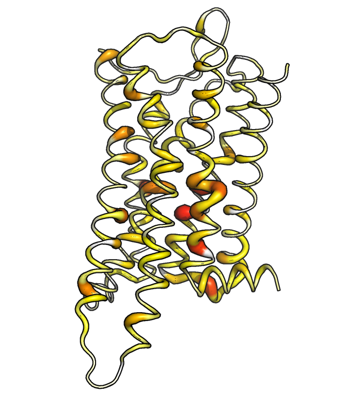
To get an overview of how strongly the ensembles differ in which region, we can plot the maximum deviation of the features related to a certain residue. The following function also writes the maximum Jensen-Shannon distance per residue in the “B factor” field of a PDB file.
ref_filename = "traj/condition-a_receptor.gro"
out_filename = "receptor_bbtors-deviations"
vis = residue_visualization(
    names_bbtors, jsd_bbtors, ref_filename,
    "plots/"+out_filename+"_jsd.pdf",
    "vispdb/"+out_filename+"_jsd.pdb",
    y_label='max. JS dist. of BB torsions'
)
Let’s now save the resulting data in CSV files.
np.savetxt(
    'results/'+out_filename+'_relen.csv',
    np.array(relen).T, fmt='%s', delimiter=',',
    header='Name, JSD(A,B), KLD(A,B), KLD(B,A)'
)
np.savetxt(
    'results/'+out_filename+'_jsd.csv',
    np.array(vis).T, fmt='%s', delimiter=',',
    header='Residue, max. JSD(A,B)'
)
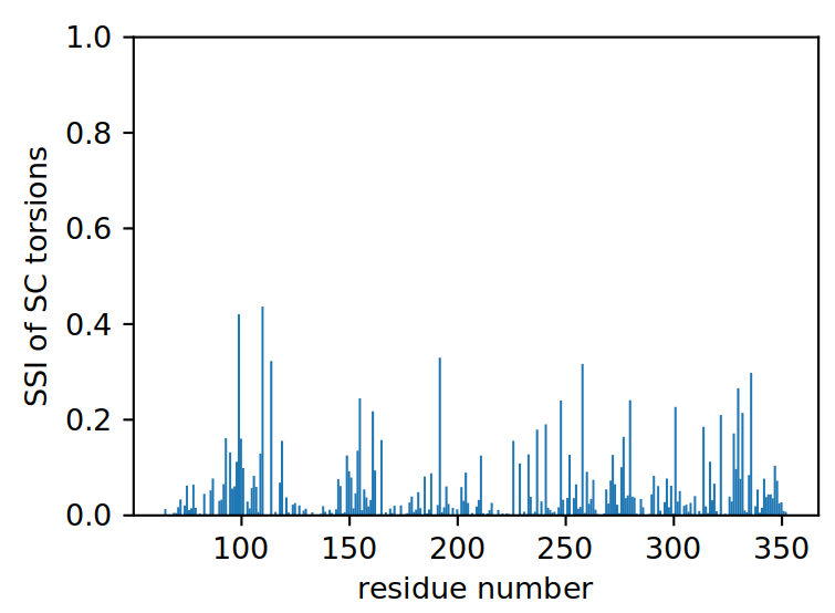
State-Specific Information
In addition, we can investigate differences in discrete conformational microstates within the torsion distributions by employing the State Specific Information (SSI) analysis in a similar manner. The prime example for this kind of analysis are protein sidechain torsions.
The conformational microstates of each residue are multidimensional, incorporating all torsion angles in the definition of a residue’s conformational space. This is why we first combine all torsions from the same residue to one multivariate feature.
multivar_res_feat_a, multivar_res_data_a = get_multivar_res(
    sim_a_rec_feat['sc-torsions'], sim_a_rec_data['sc-torsions']
)
multivar_res_feat_b, multivar_res_data_b = get_multivar_res(
    sim_b_rec_feat['sc-torsions'], sim_b_rec_data['sc-torsions']
)
Then we determine the state boundaries. The distributions are decomposed into the individual Gaussians which fit the distribution, and conformational microstates are determined based on the Gaussian intersects. It is therefore necessary that each state is sampled sufficiently in order to accurately define the conformational states.
discrete_states_ab = get_discrete_states(
    multivar_res_data_a, multivar_res_data_b
)
Now we can run the main SSI comparison.
resnames, ssi = ssi_ensemble_analysis(
    multivar_res_feat_a, multivar_res_feat_b,
    multivar_res_data_a, multivar_res_data_b,
    discrete_states_ab, verbose=False
)
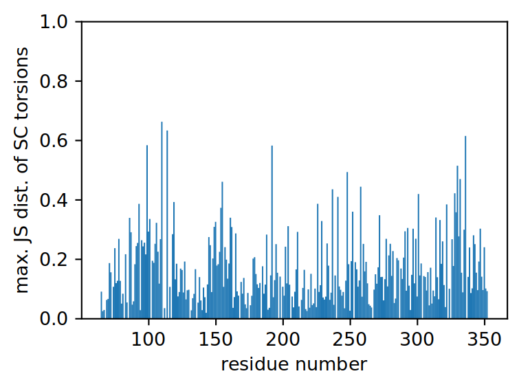
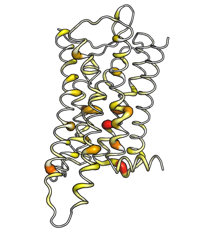
We can plot the results in the same way as we did for the backbone analysis.
ref_filename = "traj/condition-a_receptor.gro"
out_filename = "receptor_sctors-_ssi"
vis = residue_visualization(
    resnames, ssi, ref_filename,
    "plots/"+out_filename+"_ssi.pdf",
    "vispdb/"+out_filename+"_ssi.pdb",
    y_label='max. SSI of SC torsions'
)
Comparing Distances
Another common representation for the overall structure of a protein are the distances between the C-alpha atoms. We can perform the same kinds of analysis on them but will need a different approach to visualize them. Let’s use the relative entropy again:
relen = relative_entropy_analysis(
    sim_a_rec_feat['bb-distances'], sim_b_rec_feat['bb-distances'],
    sim_a_rec_data['bb-distances'], sim_b_rec_data['bb-distances'],
    bin_num=10, verbose=False
)
names_bbdist, jsd_bbdist, kld_ab_bbdist, kld_ba_bbdist = relen
We print the twelve distances with the highest deviations.
sf = sort_features(names_bbdist, jsd_bbdist)
for f in sf[:12]: print(f[0], f[1])
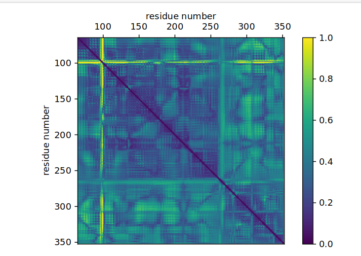
To visualize distances, we need a two-dimensional representation with the residues on each axis. We color each field with the value of the Jensen-Shannon distance (but could as well use Kullback-Leibler divergence, Kolmogorov-Smirnov statistic etc. instead).
matrix = distances_visualization(
    names_bbdist, jsd_bbdist, "plots/receptor_jsd-bbdist.pdf",
    vmin = 0.0, vmax = 1.0, cbar_label='JSD'
)