Featurization
The analysis is not performed on the coordinates directly but on features derived from these coordinates. PENSA already includes several feature readers, some of which we show here. You can also write your own following the general pattern. Note that all reader functions load the names of the features and their values separately.
Basic Example
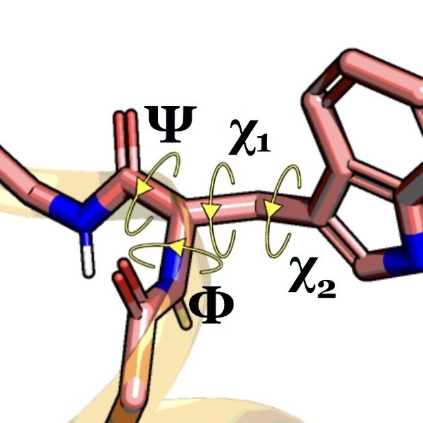
For example, we can read protein backbone torsions.
from pensa.features import *

bbtors_feat, bbtors_data = read_protein_backbone_torsions(
    "traj/condition-a_receptor.gro", "traj/condition-a_receptor.xtc",
    selection='all', first_frame=0, last_frame=None, step=1
)
The first part of the output always contains the names of the features and the second part contains the corresponding data.
print(bbtors_feat[:3])
print(bbtors_data[:3])
Having a look at the shape of the loaded data, we see that the first dimension is the number of frames. The second dimension is the number of features.
print("Number of torsions:", len(bbtors_feat))
print("Data format:", bbtors_data.shape)
PENSA has two simple functions to store features in csv file …
write_csv_features(bbtors_feat, bbtors_data, 'features/bb-torsions_a.csv')
… and to load them again.
bbtors_feat, bbtors_data = read_csv_features('features/bb-torsions_a.csv')
Protein Structure Features
Here we use the special function read_structure_features that loads
three types of structure features at once:
- backbone torsions: 'bb-torsions',
- backbone C-alpha distances: 'bb-distances', and
- sidechain torsions: 'sc-torsions'.
It was modeled after the feature loader in PyEMMA.
from pensa.features import *
sim_a_rec = read_structure_features(
    "traj/condition-a_receptor.gro",
    "traj/condition-a_receptor.xtc"
)
sim_a_rec_feat, sim_a_rec_data = sim_a_rec
sim_b_rec = read_structure_features(
    "traj/condition-b_receptor.gro",
    "traj/condition-b_receptor.xtc"
)
sim_b_rec_feat, sim_b_rec_data = sim_b_rec
For this function, the feature names and the data both contain dictionaries with entries for each feature type.
Let’s loop through them to make sure that the number of features is the same for both simulations. This is a requirement for the further analysis.
for k in sim_a_rec_data.keys():
    print(k, sim_a_rec_data[k].shape)
for k in sim_b_rec_data.keys():
    print(k, sim_b_rec_data[k].shape)
Now let’s do the same only for the transmembrane region.
sim_a_tmr = read_structure_features(
    "traj/condition-a_tm.gro",
    "traj/condition-a_tm.xtc"
)
sim_b_tmr = read_structure_features(
    "traj/condition-b_tm.gro",
    "traj/condition-b_tm.xtc"
)
sim_a_tmr_feat, sim_a_tmr_data = sim_a_tmr
sim_b_tmr_feat, sim_b_tmr_data = sim_b_tmr

for k in sim_a_rec_data.keys():
    print(k, sim_a_rec_data[k].shape)
for k in sim_b_rec_data.keys():
    print(k, sim_b_rec_data[k].shape)
Water Features
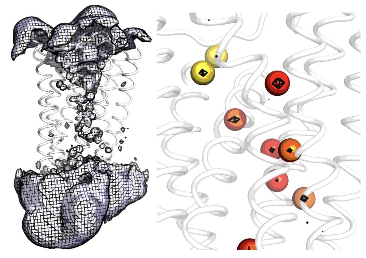
Water molecules are featurized from water density. Unlike residues which are fixed to a protein, a single water molecule can move throughout the entire simulation box, therefore featurizing a single water molecule does not make sense. Instead, it is the spatially conserved internal protein cavities in which water molecules occupy that are of interest. Water pocket featurization extracts a distribution that represents whether or not a specific protein cavity is occupied by a water molecule, and what that water molecule’s orientation (polarisation) is.
from pensa.features import *
For the pdb visualisation, the trajectory needs to be fit to the first frame of the simulation so that the density and protein align with each other.
Here we featurize the top 2 most probable water sites (top_waters = 2). Orientation of the waters (water_data - spherical coordinates [radians]) is a timeseries distribution. When water is not present at the site, the orientation is recorded as 10000.0 to represent an empty state. By specifying an name to write data out with in the argument - out_name, we can visualise the pocket occupancies on the reference structure in a pdb file with pocket occupancy saved as b_factors.
You must specify the water model for writing out the grid. options include: SPC TIP3P TIP4P water
struc = "traj/condition-a_water.gro"
xtc = "traj/condition-a_water_aligned.xtc"
water_feat, water_data = read_water_features(
    structure_input = struc,
    xtc_input = xtc,
    top_waters = 2,
    atomgroup = "OH2",
    write_grid_as="TIP3P",
    out_name = "features/11426_dyn_151_water"
)
To featurize sites common to both ensembles, we obtain the density grid following the steps in the density section of the preprocessing tutorial. This way, sites are the same across both ensembles and can be compared.
struc = "traj/condition-a_water.gro"
xtc = "traj/condition-a_water_aligned.xtc"
grid = "ab_grid_OH2_density.dx"
water_feat, water_data = read_water_features(
    structure_input = struc,
    xtc_input = xtc,
    top_waters = 2,
    atomgroup = "OH2",
    grid_input = grid
)
Single-Atom Features
For single atoms we use a similar function which provides the same functionality but ignores orientations as atoms are considered spherically symmetric.
from pensa.features import *
Here we locate the sodium site which has the highest probability. The density is written (write=True) using the default density conversion “Angstrom^{-3}” in MDAnalysis.
struc = "mor-data/11426_dyn_151.pdb"
xtc = "mor-data/11423_trj_151.xtc"
atom_feat, atom_data = read_atom_features(
    structure_input = struc,
    xtc_input = xtc,
    top_atoms = 1,
    atomgroup = "SOD",
    element = "Na",
    out_name = "features/11426_dyn_151_sodium"
)